
NASA Turbulent Flat Plate Validation Benchmark
This benchmark shows a complex CFD analysis of NASA turbulent flat plate validation using simulation environment TCAE
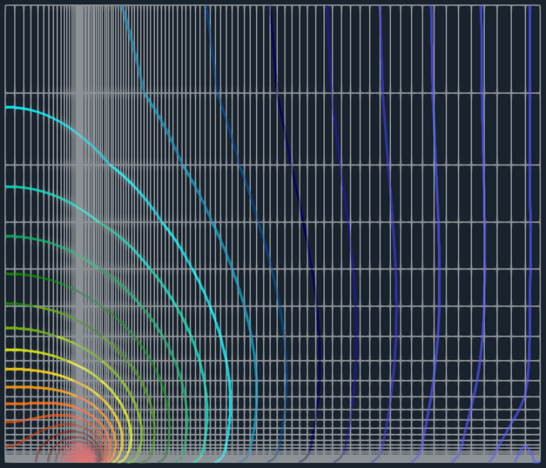
The following article is aimed at the turbulence modeling tests on a flat plate, using TCFD. This turbulent flat plate test case is well known and it has been well described on NASA website The aim of this benchmark is the validation of the turbulence models in the TCFD, computational fluid dynamics (CFD) software, and compare its results with the analytical and measurement data. The secondary aim of this test case is to compare and discuss two different wall treatments; The Low-Re modeling (resolved mesh) vs. Wall Functions modeling.
Benchmark Parameters Typical flow speed: 50 m/s Flow model: incompressible Rotation RPM: – Mesh size: 0.01/0.08M cells Impeller diameter: – mm Medium: air Reference pressure: 1 atm Typical Pressure Ratio: 0.0 Reference density: 1.2 kg/m3 Dynamic viscosity: 1.8 × 10⁻⁵ Pa⋅s Turb. Model 1: k-omega SST (WF) Turb. Model 2: v2f (Low-Re) Test Case
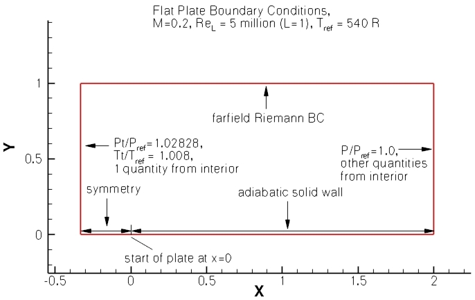
The test case topology is well described on the NASA website. It is a two-dimensional simple case sometimes called Zero Pressure Gradient Flat Plate. The flat plate is a flat wall (a line in 2d) that is being attacked by a freestream flow of 50 [m/s]. The flat plate is 2 meters long, along the x-axis, and starts in the point [0;0]. This test case is very suitable for turbulence model testing because the test case is small enough to converge quickly, and a lot of analytical and measurement data for validation is available.
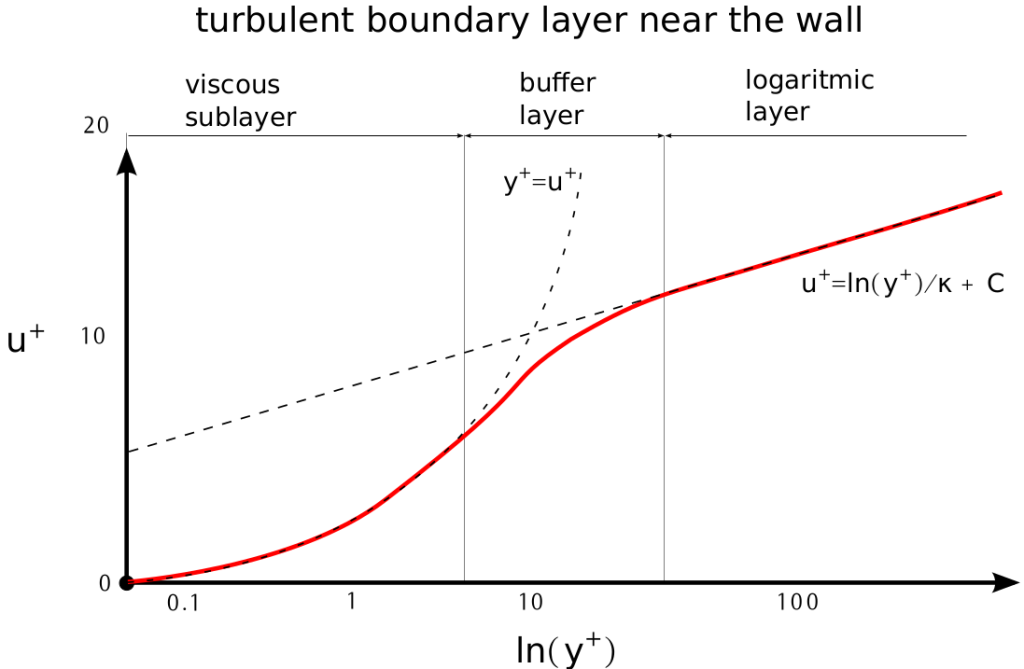
Turbulent Boundary Layer at Reθ = 10,000
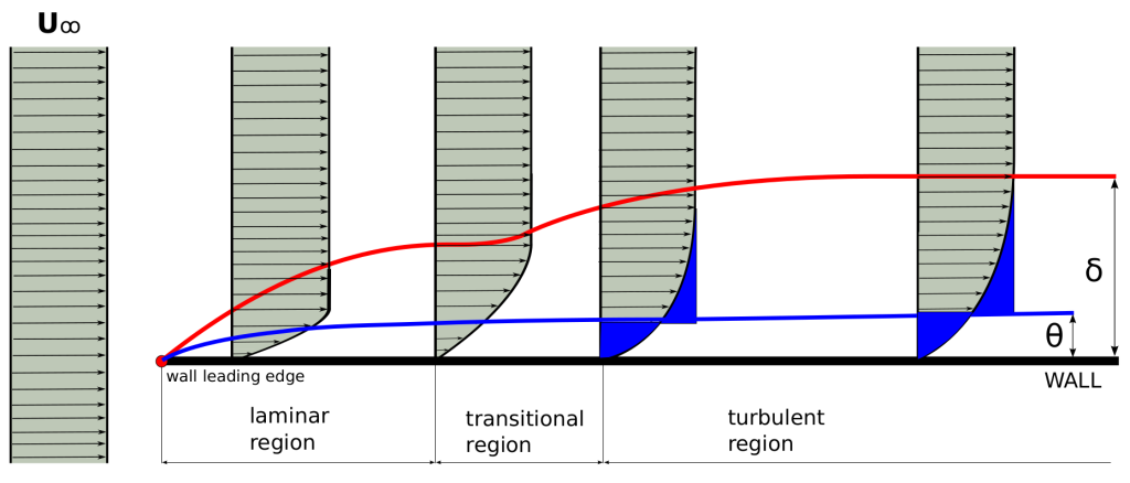
A very important characteristic of any turbulent flow is developing the turbulent boundary layer (BL). As the free stream attacks the flat plate (with zero angle of attack), the boundary layer develops along the flat plate. Three development regions can be observed; laminar region, transitional region, and turbulent region. The momentum thickness, θ, is the distance by which a surface would have to be moved parallel to itself towards the reference plane in an inviscid fluid stream of velocity U∞ to give the same total momentum as exists between the surface and the reference plane in a real fluid.
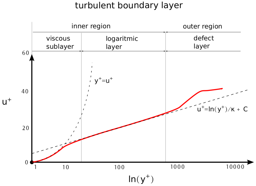
All turbulent boundary layers (BLs) on a flat plate have similar characteristics. Fully developed turbulent BL has three regions; viscous sublayer, logarithmic layer, and defect layer. To be able to compare different BLs, any BL can be displayed in dimension-less coordinates u+ and y+. Then the important part of the BL is its logarithmic layer. In the logarithmic layer the Law of the wall is valid.
The fully developed boundary layer can be viewed as divided into four regions; Viscous sublayer is a region closest to the wall. In this region, y+ = u+. The fluid flow is always laminar here. The Viscous sublayer region is typically where y + < 10. The buffer layer is a region, where no law holds and it is associated with a certain amount of uncertainty. The Buffer layer region is typically where 5 < y + < 30. Logarithmic (Log-law) layer is a region, where the Law of the wall holds. The Log-law layer region is typically where 30 < y+ < 300, and all the wall functions are trying to hit this region. Outer (Defect) layer is a region, where the free-stream is taking over. The Outer layer region is typically where 300 < y+.
Mesh
In This Particular Project, the volume meshes for the CFD simulation were created using blockMesh application. Alternatively, another external mesh can be loaded in TCFD directly in MSH, CGNS, or OpenFOAM format.

Each mesh consists of two simple blocks connected at coordinate X=0. Each mesh has a significant grading in the Y-direction and minor grading in the X-direction. All the cells are hexahedral and the test case is formally three-dimensional, but all the information in the Z-direction is completely irrelevant.
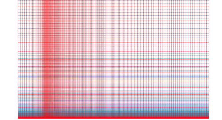
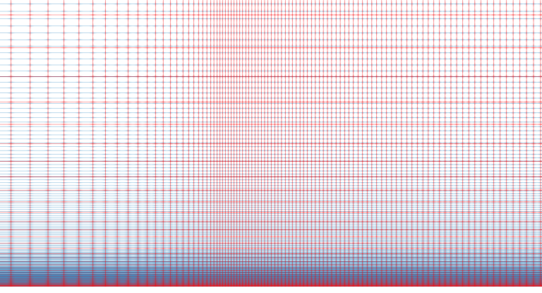
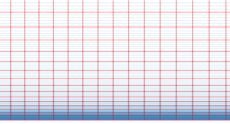
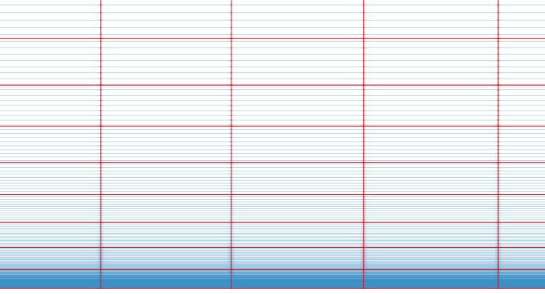
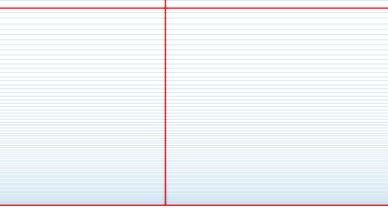
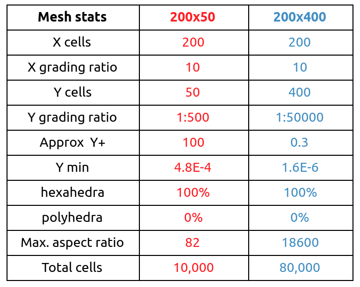
A simple bash script was used for mesh creation. For the final presentation, two meshes were created, for comparison of the wall functions method and the Low-Re method. The rough mesh 200×50 has 200 cells along the X-axis and 50 cells along the Y-axis. The fine mesh 200×400 has 200 cells along the X-axis and 400 cells along the Y-axis. These two meshes have exactly the same characteristics along the X-axis, but they differ only in the direction along Y-axis. The table below shows some selected mesh statistics:
TCFD Case Setup
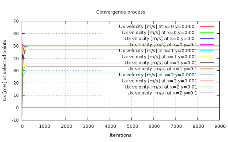
Basic TCFD settings: Machine type: stator Steady-state calculation Incompressible fluid flow RANS turbulence Model k-⍵ SST and v2f (scripted) Number of components: 1 Mesh Mesh size: 0.8M cells Inlet: Velocity 50 [m/s] Outlet: Static Pressure Speed-lines: 1 Simulation points: 1
Results - Turbulent Boundary Layer at Reθ = 10,000>
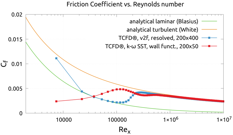
For The Final presentation, two simulations were performed in TCFD using two different methods: Case 1. Rough mesh 200×50, wall functions, with k-⍵ SST turbulence model Case 2. Fine mesh 200×400, Low-Re, with v2f turbulence model
Results - Friction Coefficient vs. ReX
Another Important aerodynamic characteristic of viscous fluid flow at a flat plate is Friction coefficient, Cf. Generally speaking, it is the ratio of the weight of an object being moved along a surface and the force that maintains contact between the object and the surface. It is defined as: Cf= 2wU2. The friction coefficient can be evaluated along the flat plate, to give us valuable information about the flow behavior. According to H. Blasius, the friction coefficient of the incompressible laminar fluid flow can be derived as: Cf= 0.664ReX, where ReX=U X . According to F. White, the friction coefficient of the incompressible turbulent fluid flow can be derived as: Cf= 0.445ln20.06 ReX For the final presentation, two simulations were performed in TCFD using two different methods: Case 1. Rough mesh 200×50, wall functions, with k-⍵ SST turbulence model Case 2. Fine mesh 200×400, Low-Re, with v2f turbulence model
Please contact us for further information.
Conclusion
- Turbulent flat plate benchmark is a very suitable test case for quick simulation tests – because, on the 2D mesh, the simulation generally converges very quickly. Case 1. shows very quick convergence (0.2 core*hours) and fully turbulent behavior everywhere along the flat plate. Case 2. shows significantly slower convergence (12 core*hours) and very high accuracy.
- All in all, the complex CFD analysis of fluid flow on the flat plate using TCFD provides very good agreement with the analytical data, as has been demonstrated.
- Potential questions will be answered on request at info@cfdsupport.com.
[1] Wilcox D.C., Turbulence Modeling for CFD , DCW Industries
[2] Stephen B. Pope, Turbulent flows. SB (2000). Cambridge Univ. Press, Cambridge.
[3] H. Versteeg, W. Malalasekera, An Introduction to Computational Fluid Dynamics: The Finite Volume Method (2nd Edition)
[4] White, Frank (2011). Fluid Mechanics. New York City, NY: McGraw-Hill. pp. 477–478. ISBN 9780071311212
[5] Prandtl, L. (1925). “Bericht uber Untersuchungen zur ausgebildeten Turbulenz”. Zeitschrift fur angew. Math. u. Mechanik
[6] https://en.wikipedia.org/wiki/Skin_friction_drag
Download TCAE Tutorial - Flat Plate Benchmark
File name: flatPlate-TCAE-Tutorial-21.09.zip
File size: 0.1 MB
Tutorial Features: CFD, TCAE, TMESH, TCFD, TFEA, SIMULATION, RANS, AUTOMATION, WORKFLOW, RADIAL FLOW.
