1

Previous: castellatedMeshControls Up: SnappyHexMesh mesh Next: addLayersControls

This is an automatically generated documentation by LaTeX2HTML utility. In case of any issue, please, contact us at info@cfdsupport.com.

SnapControls

This block defines parameters for snapping, i.e., process for mesh alignment with the geometry.

    // Number of patch smoothing iterations before finding correspondence
    // to surface
    nSmoothPatch 3;

    // Maximum relative distance for points to be attracted by surface.
    // True distance is this factor times local maximum edge length.
    // Note: changed(corrected) w.r.t 17x! (17x used 2* tolerance)
    tolerance 2.0;

    // Number of mesh displacement relaxation iterations.
    nSolveIter 30;

    // Maximum number of snapping relaxation iterations. Should stop
    // before upon reaching a correct mesh.
    nRelaxIter 5;

    // Feature snapping

        // Number of feature edge snapping iterations.
        // Leave out altogether to disable.
        nFeatureSnapIter 10;

        // Detect (geometric only) features by sampling the surface
        // (default=false).
        implicitFeatureSnap false;

        // Use castellatedMeshControls::features (default = true)
        explicitFeatureSnap true;

        // Detect features between multiple surfaces
        // (only for explicitFeatureSnap, default = false)
        multiRegionFeatureSnap false;
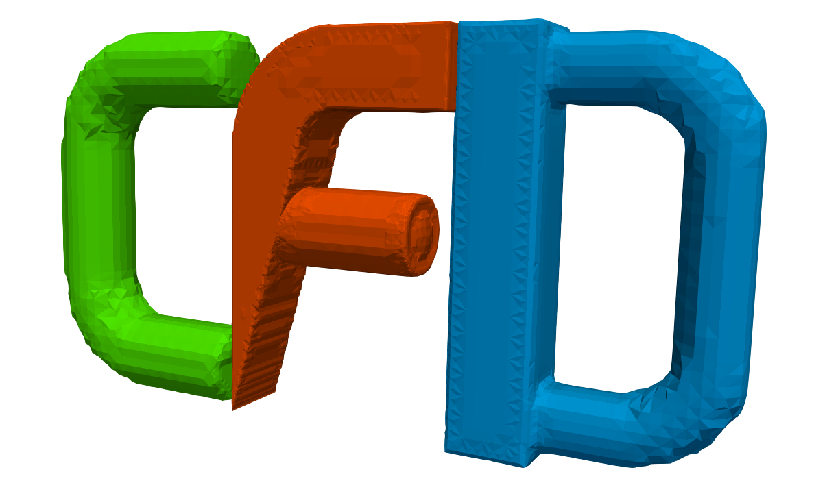
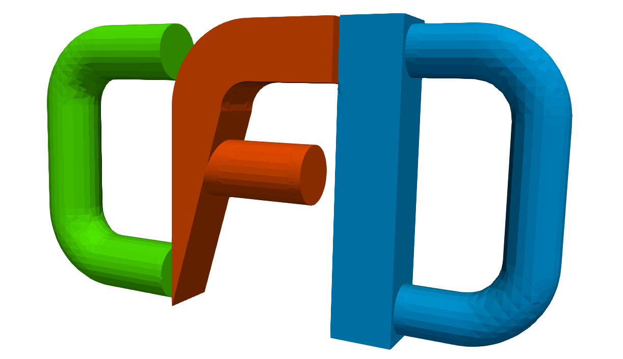
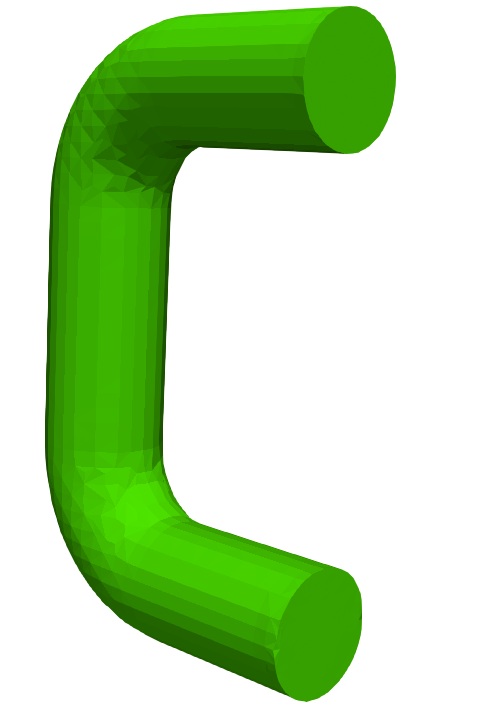
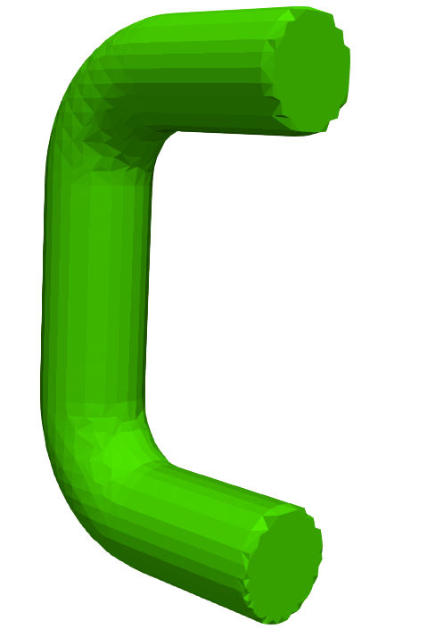
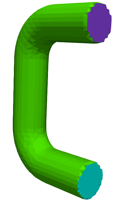
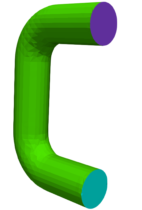
  • tolerance – relative distance for points to be attracted by surface, example of two different setups is visualized in Figure crossref 2
snappyTolerance01 1
snappyTolerance20 1

Figure: tolerance: 0.1 vs 2.0; objects surface visualization.

  • implicitFeatureSnap – snaps to automatically detected feature edges following the resolveFeatureAngle parameter
  • explicitFeatureSnap – snaps to manually generated feature edges, reads the features block
  • multiRegionFeatureSnap – snaps to automatically detected boundary edges of each item in refinementSurfaces block
  • Example of different setups is depicted in Figure crossref 2

false-false-false

snappyFeatureSnapFFF

true-false-false

snappyFeatureSnapTFF

false-true-false

snappyFeatureSnapFTF

Figure: implicit*, explicit*, multiRegion* – FeatureSnap combinations.

  • The multiRegionFeatureSnap make sense if your object is defined using several separte STLs.
  • It is possible to split your object (one STL file) using utilities surfaceAutoPatch and surfaceSplitByPatches:
    • Go to constant/triSurface directory and run following commands:
      # surfaceAutoPatch C-fine.stl C-fine-split.stl 130
      # surfaceSplitByPatch C-fine-split.stl
    • The number 35 is similar to includedAngle parameter in surfaceFeatureExtractDict:
      • 36 – no splitting of the surface
      • 37 – any triangle will be split into separate patch
    • It generates three separate files which can be used for mesh generation, you can update the snappyHexMeshDict in the following way:
      geometry
      {
          C-fine-split_patch0.stl
          {
              type triSurfaceMesh;
              name C0;
          }
          C-fine-split_patch1.stl
          {
              type triSurfaceMesh;
              name C1;
          }
          C-fine-split_patch2.stl
          {
              type triSurfaceMesh;
              name C2;
          }
          F-fine.stl
          {
              type triSurfaceMesh;
              name F;
          }
      
          refinementSurfaces
          {
              "C-*"          
              { 
                  level (2 2); 
                  patchInfo 
                  { 
                      type wall;                
                  }            
              }
      
          layers
          {
              "C[0-9]" 
              {
                  nSurfaceLayers  3;
                  expansionRatio  1.5;
              }
      
    • In refinementSurfaces and layers blocks it is allowed to use regular expressions.
    • Now we can test different setups of multiRegionFeatureSnap, see Figure crossref 2. It clearly shows, that multiRegionFeatureSnap is enabled only when explicitFeatureSnap is enabled as well.

false-false-false

snappyFeatureSnapFFF 1

false-false-true

snappyFeatureSnapFFT

false-true-true

snappyFeatureSnapFTT

Figure: implicit*, explicit*, multiRegion* – FeatureSnap combinations.

OpenFOAM Directories

OpenFOAMBasic Directory
img256 1 OpenFOAM-2.x.xDirectory with OpenFOAM version 2.x.x
     img256 1 applicationsApplications and their sources
     img256 1 binScripts for compiler
     img256 1 docDocumentation
     img256 1 etcConfiguration files
     img256 1 platformsShared libraries
         img256 1 platformName= architecture+compiler+precission+options
             img256 1 binScripts and application binary files
             img256 1 libBinary files of libraries
     img256 1 srcSource code of libraries
     img256 1 tutorialsTutorials – preset test cases
     img256 1 wmakeDirectives for compiler

Previous: Example: Pressure around the Up: Example: Pressure around the Next: Example: Blade pressure and
This is an automatically generated documentation by LaTeX2HTML utility. In case of any issue, please, contact us at info@cfdsupport.com.

Step by step guide

Step 1 — Load the rotor part of an OpenFOAM case into ParaView using the command paraFoam -region rotor. Avoid loading the whole mesh; choose only the blade walls and the hub and shroud patches. Choose some non-zero simulation time, select appropriate components (“Mesh parts”) and fields (“Volume fields”) and press “Apply”. This will load the necessary patches, figure [*].

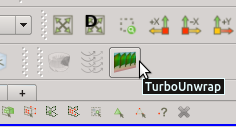
Step 2 — First, the blades need to be transformed from the cylinder- or disk-like arrangement to a straight rectangular block. This is done by the filter Turbo Unwrap. You should see the icon of the filter in the toolbar. Note that the filter is available (i.e. coloured and clickable) only when the data selected in “Pipeline browser” are of the type “Multi-block Dataset” (see panel “Information”, section “Statistics”).

23

Either use this button, or select the filter Turbo Unwrap in the Filters > Turbomachinery (or Filters > Alphabetical) menu, or use the search box from Filters > Search. This will add the filter into the “Pipeline browser”.

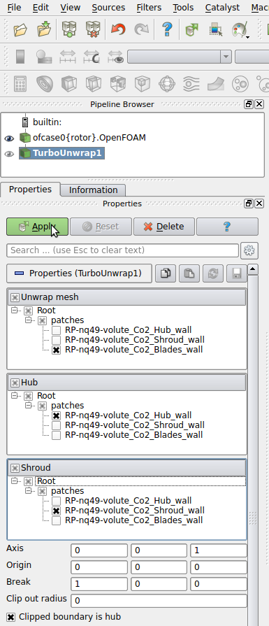
Step 3 — The basic properties of the filter Turbo Unwrap are shown in the figure [*]. When the advanced options are hidden, there are only a few options to define. First of all, it is necessary to choose the blade wall patch, that will be transformed, and the hub and shroud patches, which will serve as a leaders to define the transformation. After the transformation is done, hub and shroud will be perfectly flat and parallel to each other, conformly deforming the mesh in between. If multiple mesh parts are selected in the “Unwrap mesh” window or multiple patches are selected in “Hub” or “Shroud” windows then they will be internally merged into a single entity before proceeding. In this example the mesh is well prepared and we can just select the three items that we loaded in the first step.
Step 4 — Set the direction and position of the rotating axis using the parameters “Axis” and “Origin”. In our case we use $ z$-axis, which is the default option.

Step 5 — Unlike in the case of the blade-to-blade view, when constructing the pressure profile it is mostly not necessary to specify a non-zero “Clip out radius”, because the blades do not reach all the way to the axis in the middle. We will leave the parameter having its default zero value.

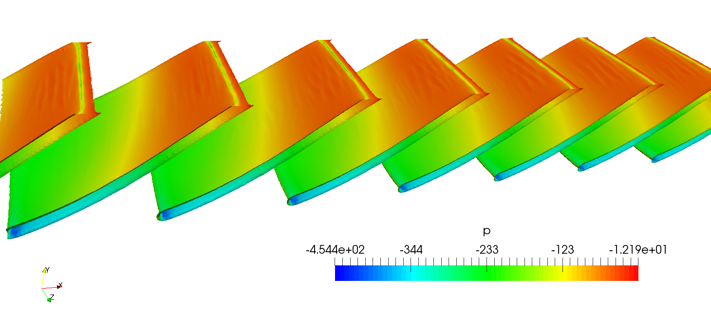
Step 6 — Click on “Apply”. The transformation should be relatively fast, because the sufrace mesh of the blades is orders of magnitude easier to process than the full volume mesh. It may be necessary to zoom in or out a little (depending on the geometry) to make the result fit to window. Outcome of this step is shown in the figure [*], where the blades are coloured by pressure.
Step 7 — Having the blades transformed we can now cut them at a specific height ($ z$-axis) using the filter Slice. This will result in several two-dimensional intersection contours.
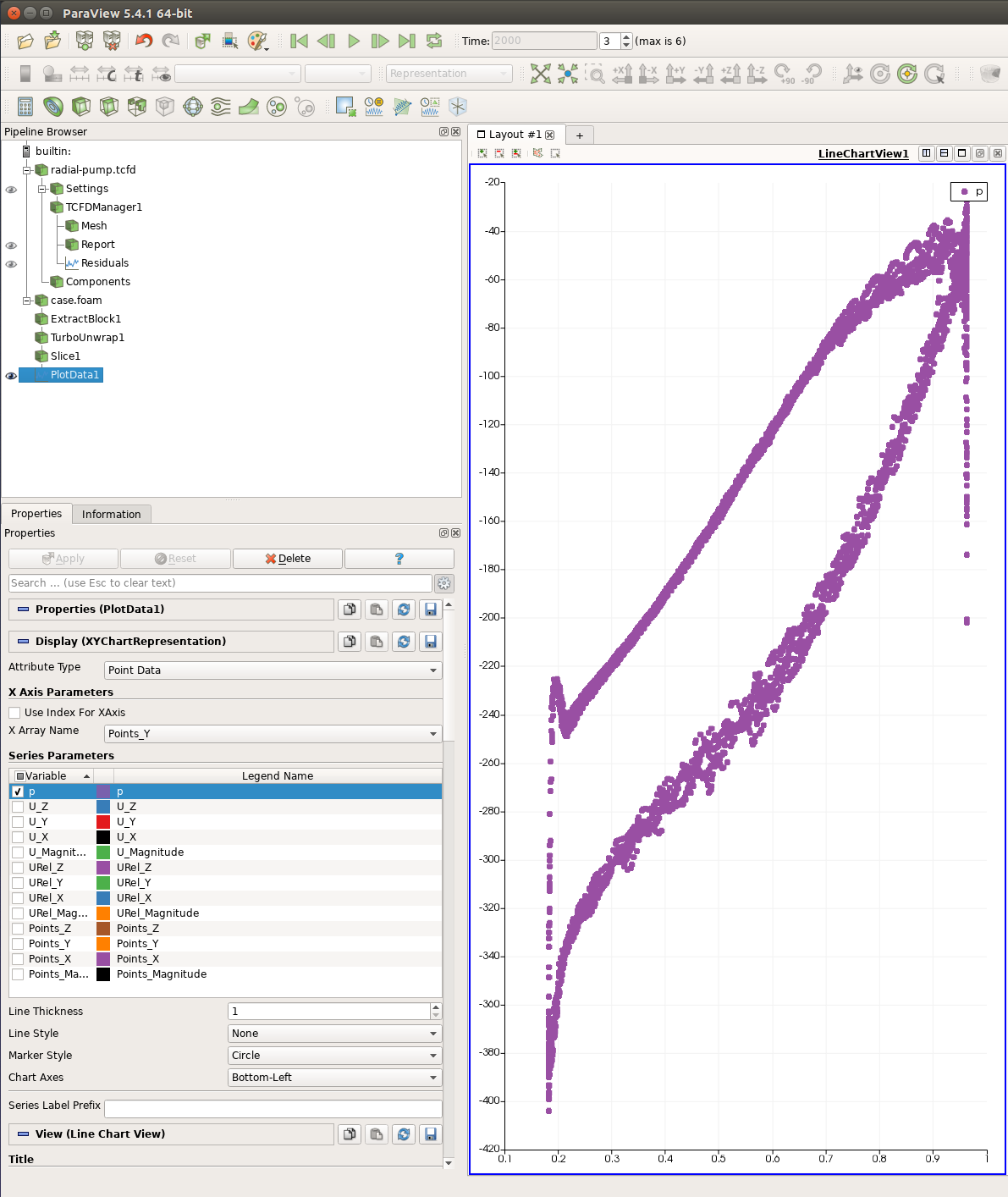
Step 8 — Add the filter Plot Data from Filters > Alphabetical or using Filters > Search. Unselect all fields but pressure (see figure [*]). Above the field selection box use “Points_Y” as the “X Array Name”. This will use points’ Y coordinates as the data for the horizontal axis. Below the field selection box use “None” as “Line Style” and “Circle” as “Marker Style”. This will only show one bullet per a mesh point, making the result independent on the order of the projected points. Now press “Apply”. You should obtain a similar figure to [*].
24

Figure: Settings of the Turbo Blade Post / Turbo Unwrap filter for transformation of blades of the pump.

Note — The plot will contain data from all blades. As the blades are equivalent, it doesn’t hurt the visualization. If just a single blade profile was required, it would be necessary to separate one of the contours using a pair of the Clip filters .

turbo blade post turbo unwrap blade unwrapped
26

Figure: Pressure distribution around the blade for a given height (i.e. relative distance from the hub to the shroud) constructed with the aid of the plugins of Turbo Blade Post toolset. The horizontal axis shows the transformed Y axis, which corresponds to the normalized inlet-to-outlet direction position (for given hub-to-shroud distance and angular position). The vertical axis displays the value of the pressure as computed by TCFD using OpenFOAM.