Previous: Example: Blade-to-blade view Up: Example: Blade-to-blade view Next: Example: Pressure around the
This is an automatically generated documentation by LaTeX2HTML utility. In case of any issue, please, contact us at info@cfdsupport.com.
Step by step guide
![Node125 7 [*]](https://www.cfdsupport.com/wp-content/uploads/2022/02/crossref.png) left), or “Read Zones” check-box below to read the rotating zone (figure
left), or “Read Zones” check-box below to read the rotating zone (figure ![Node125 7 [*]](https://www.cfdsupport.com/wp-content/uploads/2022/02/crossref.png) right). The former way, more frequent in Linux, will add available zones at the end of the “Mesh Parts” selection list (and you need to select them manually). The latter way, more frequent in Windows, will automatically read all available zones after clicking on the “Apply” button. Choose some non-zero simulation time, select appropriate components (“Mesh parts”) and fields (“Volume fields”) and press “Apply”. This will load the mesh.
right). The former way, more frequent in Linux, will add available zones at the end of the “Mesh Parts” selection list (and you need to select them manually). The latter way, more frequent in Windows, will automatically read all available zones after clicking on the “Apply” button. Choose some non-zero simulation time, select appropriate components (“Mesh parts”) and fields (“Volume fields”) and press “Apply”. This will load the mesh. ![Node125 7 [*]](https://www.cfdsupport.com/wp-content/uploads/2022/02/crossref.png) or
or ![Node125 7 [*]](https://www.cfdsupport.com/wp-content/uploads/2022/02/crossref.png) ) into the normalized rectangular block can be calculated by the filter Turbo Unwrap. You should see the icon of the filter in the toolbar. Note that the filter is available (i.e. coloured and clickable) only when the data selected in “Pipeline browser” are of the type “Multi-block Dataset” (see panel “Information”, section “Statistics”).
) into the normalized rectangular block can be calculated by the filter Turbo Unwrap. You should see the icon of the filter in the toolbar. Note that the filter is available (i.e. coloured and clickable) only when the data selected in “Pipeline browser” are of the type “Multi-block Dataset” (see panel “Information”, section “Statistics”). 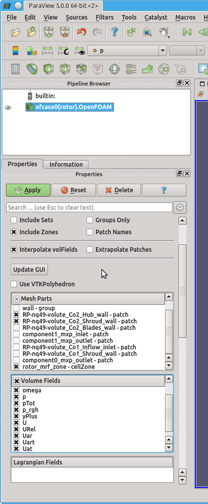
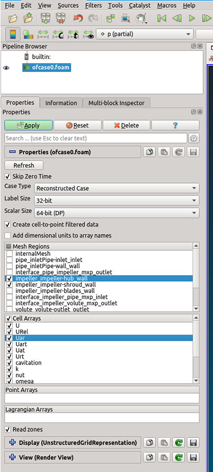
Figure: Loading mesh zones and the hub and shroud patches needed by the filter Turbo Unwrap. Left (OpenFOAM’s OpenFOAM reader): Hub and shroud patches are selected, as well as the rotating zone. Right (ParaView’s Foam reader): Hub and shroud patches and all zones are selected.
Step 3 — The basic properties of the filter Turbo Unwrap are shown in the figure ![Node125 7 [*]](https://www.cfdsupport.com/wp-content/uploads/2022/02/crossref.png) . When the advanced options are hidden, there are only a few options to define. First of all, it is necessary to choose the internal mesh, that will be transformed, and the hub and shroud patches, which will serve as a leaders to define the transformation. After the transformation is done, hub and shroud will be perfectly flat and parallel to each other, conformly deforming the mesh in between. If multiple mesh parts are selected in the “Unwrap mesh” window or multiple patches are selected in “Hub” or “Shroud” windows then they will be internally merged into a single entity before proceeding. In this example the mesh is well prepared and we can just select the three items that we loaded in the first step.
. When the advanced options are hidden, there are only a few options to define. First of all, it is necessary to choose the internal mesh, that will be transformed, and the hub and shroud patches, which will serve as a leaders to define the transformation. After the transformation is done, hub and shroud will be perfectly flat and parallel to each other, conformly deforming the mesh in between. If multiple mesh parts are selected in the “Unwrap mesh” window or multiple patches are selected in “Hub” or “Shroud” windows then they will be internally merged into a single entity before proceeding. In this example the mesh is well prepared and we can just select the three items that we loaded in the first step.
![Node125 7 [*]](https://www.cfdsupport.com/wp-content/uploads/2022/02/crossref.png) . The nature of the transformation is illustrated in the figures
. The nature of the transformation is illustrated in the figures ![Node125 7 [*]](https://www.cfdsupport.com/wp-content/uploads/2022/02/crossref.png) –
–![Node125 7 [*]](https://www.cfdsupport.com/wp-content/uploads/2022/02/crossref.png) .
. Step 7 — Unlike the scalar quantities (like pressure) the vector fields need to be transformed, too, when the mesh transforms. This is done automatically for the cell fields U and URel. As a by-product the filter also produces several other cell fields that can be used as an input to other filters: The local streamline vectors UStream and URelStream, and the cell field URelLIC, which is particularly well suited for usage in Line Integral Convolution (“SurfaceLIC”) representation. To use these fields in filters that request point fields, it is necessary to interpolate the data from points to cells, which is done as the final step using the filter Cell data to point data (can be found in Filters > Alphabetical). This filter has no important settings.
![Node125 7 [*]](https://www.cfdsupport.com/wp-content/uploads/2022/02/crossref.png) , the resulting cut displaying pressure is the figure
, the resulting cut displaying pressure is the figure ![Node125 7 [*]](https://www.cfdsupport.com/wp-content/uploads/2022/02/crossref.png) , or showing the SurfaceLIC representation (with settings from
, or showing the SurfaceLIC representation (with settings from ![Node125 7 [*]](https://www.cfdsupport.com/wp-content/uploads/2022/02/crossref.png) ) in the figure
) in the figure ![Node125 7 [*]](https://www.cfdsupport.com/wp-content/uploads/2022/02/crossref.png) .
. 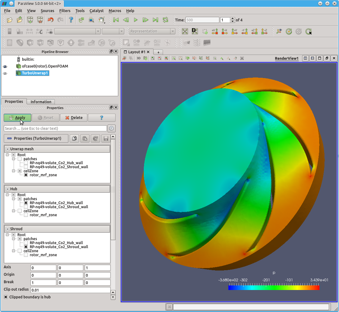
Figure: Basic parameters of the filter Turbo Unwrap.
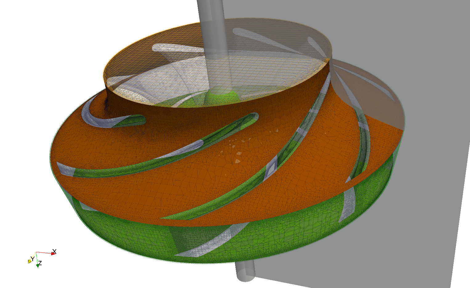
Figure: Rotating area of the simulated pump’s volume before the application of the filter Turbo Unwrap. The patches are coloured here to make them easily differentiable in the following figure [![]() ]. Hub patch (bottom) is in solid green, shroud patch (top) in solid orange, inflow (top) is orange wireframe and outflow (bottom) green wireframe. The figure also contains the clipping cylinder corresponding to the parameter “Clip out radius” and the cutting semiplane corresponding to the direction specified by the parameter “Break”.
]. Hub patch (bottom) is in solid green, shroud patch (top) in solid orange, inflow (top) is orange wireframe and outflow (bottom) green wireframe. The figure also contains the clipping cylinder corresponding to the parameter “Clip out radius” and the cutting semiplane corresponding to the direction specified by the parameter “Break”.
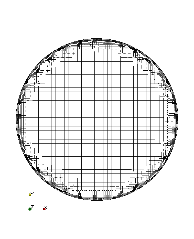
Figure: Detail of the inflow interface mesh structure of the pump test case before the application of Turbo Blade Post plugin Turbo Unwrap.
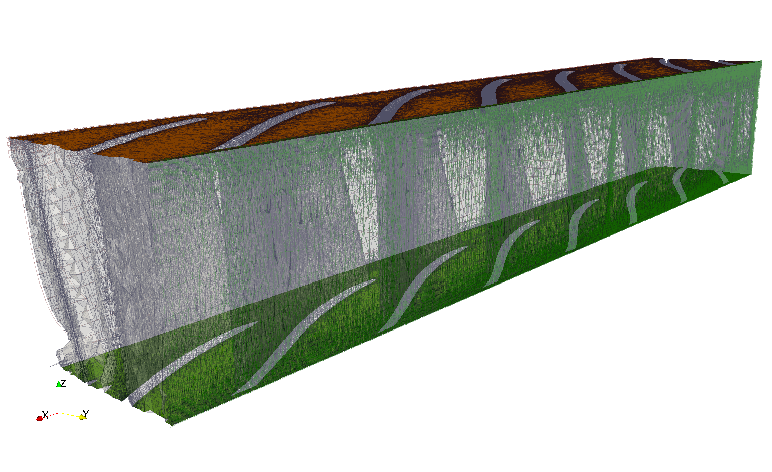
 , the normalized circular coordinate is transformed to
  and the remaining coordinate that is orthogonal to both, “along the stream”, is mapped to
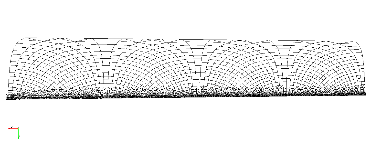
Figure: Detail of the inflow interface mesh structure of the pump test case after the application of Turbo Blade Post plugin Turbo Unwrap.
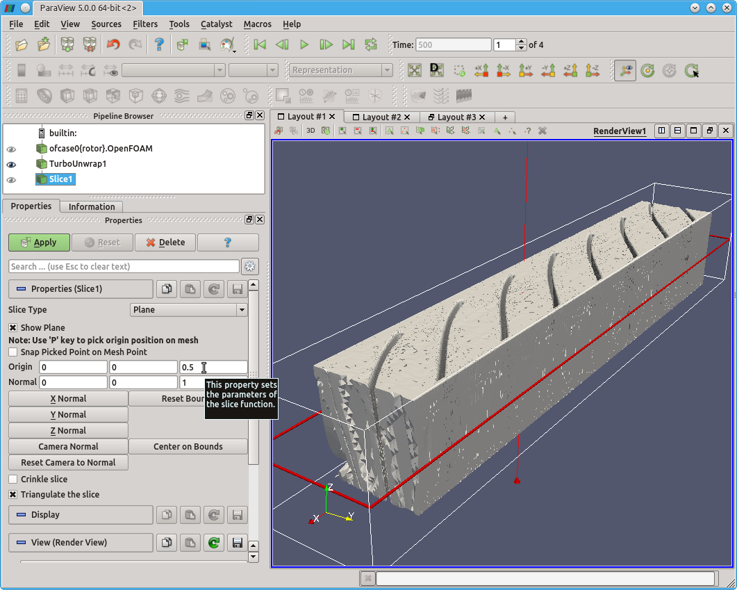
Figure: Construction of the blade-to-blade view from the rotor block unwrapped by Turbo Blade Post plugin Turbo Unwrap.
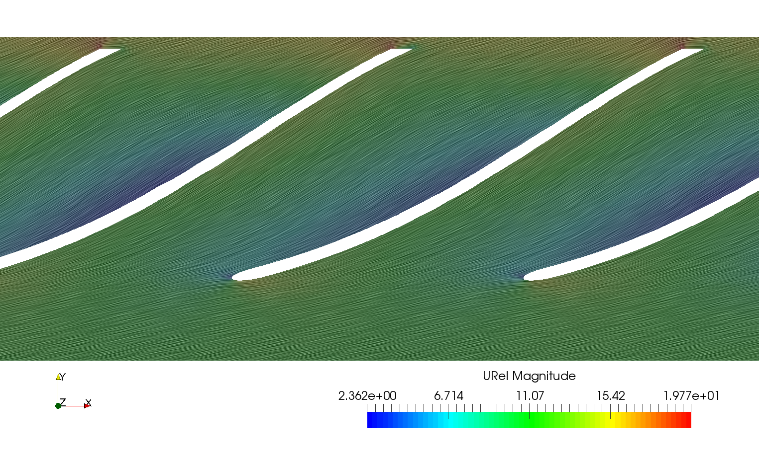
Figure: Construction of the blade-to-blade view from the rotor block unwrapped by Turbo Blade Post plugin Turbo Unwrap.
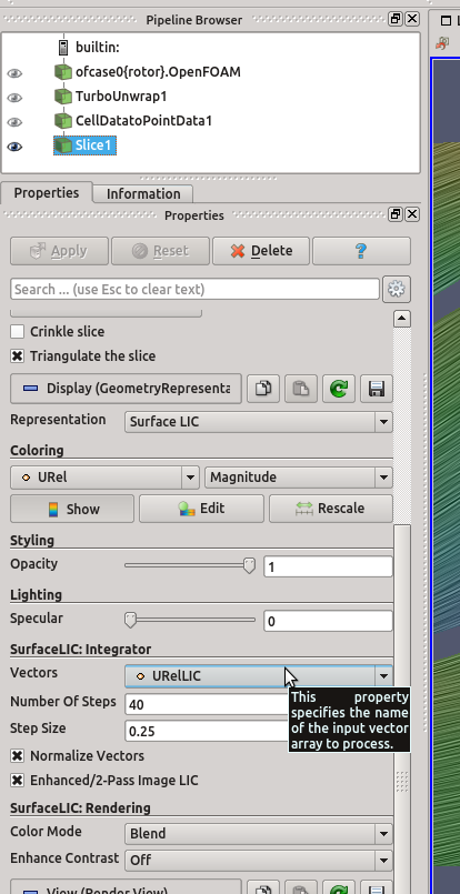
Figure: Surface Line Integral Convolution setup after application of Turbo Unwrap + Cell Data To Point Data filters. The coloring is taken from the magnitude of the vector field URel, the directions and sizes from URelLIC.


