Previous: Example: Pressure around the Up: Example: Pressure around the Next: Example: Blade pressure and
This is an automatically generated documentation by LaTeX2HTML utility. In case of any issue, please, contact us at info@cfdsupport.com.
Step by step guide
![Node127 7 [*]](https://www.cfdsupport.com/wp-content/uploads/2022/02/crossref.png) .
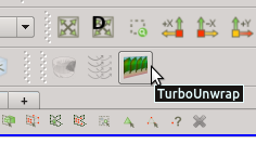
. Step 2 — First, the blades need to be transformed from the cylinder- or disk-like arrangement to a straight rectangular block. This is done by the filter Turbo Unwrap. You should see the icon of the filter in the toolbar. Note that the filter is available (i.e. coloured and clickable) only when the data selected in “Pipeline browser” are of the type “Multi-block Dataset” (see panel “Information”, section “Statistics”).
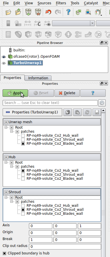
![Node127 7 [*]](https://www.cfdsupport.com/wp-content/uploads/2022/02/crossref.png) . When the advanced options are hidden, there are only a few options to define. First of all, it is necessary to choose the blade wall patch, that will be transformed, and the hub and shroud patches, which will serve as a leaders to define the transformation. After the transformation is done, hub and shroud will be perfectly flat and parallel to each other, conformly deforming the mesh in between. If multiple mesh parts are selected in the “Unwrap mesh” window or multiple patches are selected in “Hub” or “Shroud” windows then they will be internally merged into a single entity before proceeding. In this example the mesh is well prepared and we can just select the three items that we loaded in the first step.
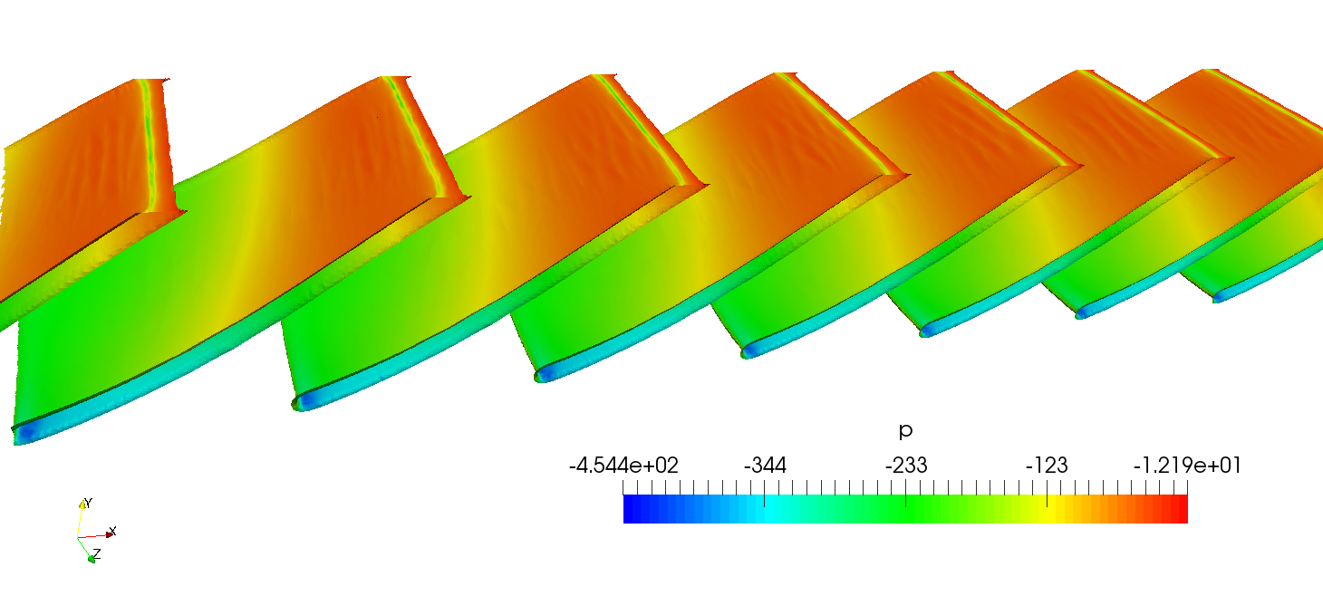
. When the advanced options are hidden, there are only a few options to define. First of all, it is necessary to choose the blade wall patch, that will be transformed, and the hub and shroud patches, which will serve as a leaders to define the transformation. After the transformation is done, hub and shroud will be perfectly flat and parallel to each other, conformly deforming the mesh in between. If multiple mesh parts are selected in the “Unwrap mesh” window or multiple patches are selected in “Hub” or “Shroud” windows then they will be internally merged into a single entity before proceeding. In this example the mesh is well prepared and we can just select the three items that we loaded in the first step. ![Node127 7 [*]](https://www.cfdsupport.com/wp-content/uploads/2022/02/crossref.png) , where the blades are coloured by pressure.
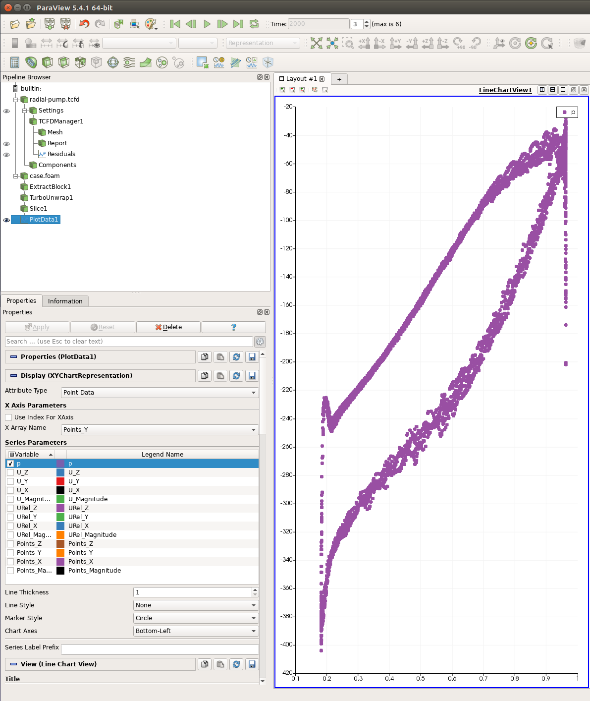
, where the blades are coloured by pressure. ![Node127 7 [*]](https://www.cfdsupport.com/wp-content/uploads/2022/02/crossref.png) ). Above the field selection box use “Points_Y” as the “X Array Name”. This will use points’ Y coordinates as the data for the horizontal axis. Below the field selection box use “None” as “Line Style” and “Circle” as “Marker Style”. This will only show one bullet per a mesh point, making the result independent on the order of the projected points. Now press “Apply”. You should obtain a similar figure to
). Above the field selection box use “Points_Y” as the “X Array Name”. This will use points’ Y coordinates as the data for the horizontal axis. Below the field selection box use “None” as “Line Style” and “Circle” as “Marker Style”. This will only show one bullet per a mesh point, making the result independent on the order of the projected points. Now press “Apply”. You should obtain a similar figure to ![Node127 7 [*]](https://www.cfdsupport.com/wp-content/uploads/2022/02/crossref.png) .
. 
Figure: Settings of the Turbo Blade Post / Turbo Unwrap filter for transformation of blades of the pump.


Figure: Pressure distribution around the blade for a given height (i.e. relative distance from the hub to the shroud) constructed with the aid of the plugins of Turbo Blade Post toolset. The horizontal axis shows the transformed Y axis, which corresponds to the normalized inlet-to-outlet direction position (for given hub-to-shroud distance and angular position). The vertical axis displays the value of the pressure as computed by TCFD using OpenFOAM.


