Beam-Ball FSI Simulation Benchmark

This report presents the FSI (Fluid-Structure Interaction) validation benchmark, using TCAE simulation software. This study is unique, because the exact solution can be evaluated analytically, and the analytical solution can be compared with the simulation results. The particular goal of this study is to investigate and compare the deformation of a beam with a ball at its end, stressed by the airflow.

Beam-Ball Benchmark Introduction

This Study is Unique , because the exact solution can be evaluated analytically, and the analytical solution can be compared with the simulation results. The particular goal of this benchmark is to investigate and compare the deformation of a beam with a ball at its end, stressed by the airflow. Let’s consider the following case as shown in the simple sketch below:

The ball (sphere),with diameter D = 30 cm, is closely fixed to the beam (cylindrical rod), with length L = 1 m and diameter d = 1 cm, which is fixed in the wall. The beam and ball material is steel. The beam-ball system is exposed to the airflow, which velocity is U∞=30 m/s. The airflow acts on the beam-ball system and the beam bends due to the aerodynamic force. Let’s determine the beam deformation (displacement at the free end of the beam where the ball is fixed). The other objective is finding the material stress distribution, particularly, the maximal stress (to be able to compare results from 1D analysis to 3D simulation results). This task can be solved both analytically, and numerically using special CAE software.

The analytical solution can be done per-partes. First, the aerodynamics drag force, which is acting on the ball, can be evaluated from a physical formula (and double-checked with the simulation).

Second, the resulting aerodynamic drag force is used as a point load at a 1D analysis of a cantilever beam, fixed in the wall.

The correctness of the 1D analysis below can be also verified with the quick online cantilever beam calculator e.g. at https://calcresource.com/statics-cantilever-beam.html.

Ball Aerodynamics - Drag Force Analytical solution

The drag force acting on object can determined by a simple formula:

F = 0.5 · Cd · Aref · ρ · U∞^2

where
● A is a reference area, in our case it is an area of a circle with the same diameter as a sphere
● ρ is density of fluid
● U∞ is velocity of mean fluid flow
● Cd is drag coefficient

Ball Aerodynamics - Sphere Drag Force Analytical Solution

Drag coefficient of the ball The drag coefficient, Cd, of the ball (sphere) is depending on the Reynolds Number [4]

Re = (ρ · U∞ · D) / μ = 50 000

The estimation of the ball drag coefficient is not straightforward. Considering the Reynolds number of 50000, according to NASA documentation at https://www.grc.nasa.gov/www/k-12/airplane/dragsphere.html, the drag coefficient can be estimated in a range from Cd = 0.1-0.5, which leads to evaluating the drag force acting on the ball to:

F = 0.5 · Cd · Aref · ρ · U∞2 ≃ 3.807 – 19.035 [N]

The CFD simulation, described below, gives the drag coefficient, Cd = 0.19, which leads to the drag force:

F ≃ 8.22462 [N]

Beam Deformation Analytical Solution

Let’s consider a simplified one-dimensional model of a cantilever beam, with one fixed end and one free end. Let the beam length is L and the beam is loaded with a single point load (force F) at its end.

We can obtain analytical solution of beam displacement, δ , anywhere along the beam by (x) applying Mohr integral formula

δ (x) = 1/EI ∫(L) Mo(x) · mo(x) dx [m]

Where
● Mo(x) denotes Bending Moment Function, along the beam length (x – coordinate, x=0 at o the free end and x=L at the wall), from load by the force F
● mo(x) means Bending Moment, along the beam length (x – coordinate, x=0 at the free end and x=L at the wall), from unit dimensionless force (“1”) applied at the very point, where we want to analyse displacement
● E is Young Modulus of Elasticity of the beam material
● I represents the Moment of Inertia of a beam cross-section. For circular beams it is

I = π·d^4 / 64

In our particular case, the moment functions are

Mo(x) = F · x

mo(x) = “1” · x

Which gives us integral

δ(x) = 1/EI ∫{0-L} F · x^2 dx

After integration we obtain

δ = 1/EI [F·x^3/3]{0-L} = 1/EI [F·L^3/3]

Which can be simplified into a form

δ = 0.003234 · F = 0.026598 [m]

Beam Stress - Analytical solution

Let’s consider the same cantilever beam ,with one fixed end and one free end. Let the beam length is L and the beam is loaded with a single point load (force F) at its end.

Now we derive the material stress in the beam

σo(x) = Mo(x)/Wo [Pa]

where

● σo(x) is the Stress Function, along the beam length (x – coordinate, x=0 at the free end and x=L at the wall), from load by the force F
● Mo(x) denotes Bending Moment Function, along the beam length (x – coordinate, x=0 at the free end and x=L at the wall), from load by the force F
● Wo declares Resistant Moment of the neutral axis of bending, which is Moment of Inertia divided by the longest distance of thread from the neutral axis, in our case of circular beam it is

Wo = I/y = π·d^4/64 / d/2 = π·d^3/32 = 9.8172E−8 [m3]

In the structural analysis, we are typically interested in the maximal value of the stress. That can be found by the derivation of stress or moment function to find maximal or minimal values

∂x/∂σo(x) = 0

In our model, we can simply assume, that the stress function is linear and the maximal stress will be at the wall ( x = L ), so

σomax = Mo(x = L)/Wo = F·L/Wo

σomax = 1.0186E−7 · F = 8.3776E−7 [Pa]

Beam-Ball Full Case Simulation in TCAE

The beam ball surface model is created in CAD and loaded in TCAE in the form of fine 3D STL surface files. All the simulation setup is done in the TCAE graphical interface.

The TCAE simulation workflow is completely automated. If the simulation setup is completed, the whole simulation process is run with a single click of the Run all button in GUI or s single command is executed in the command line.

TCAE consists of different software modules. The simulation workflow chronological order is following:

Start -> CFD mesh -> FEA mesh -> CFD simulation -> FSI -> FEA simulation -> Report

This Particular case uses following TCAE software modules: TMESH module creates meshes both for CFD and FEA and makes them ready for the simulation. TCFD module runs CFD simulation and writes down the CFD results report. TFEA module makes FSI conversion, runs FEA simulation, and writes down the FEA results report.

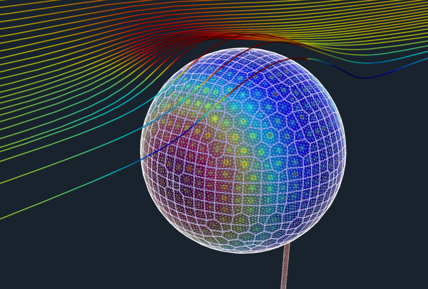
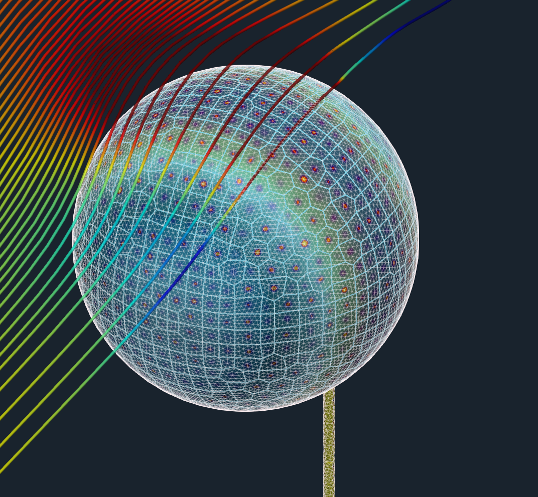
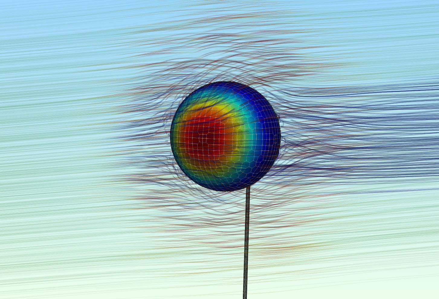
The aerodynamic effects acting on the beam itself are neglected. The aerodynamic simulation is performed only around the ball (sphere) to benefit from completely symmetrical mesh to receive as accurate results as possible. Note, the simulation results will be compared with an analytical solution, which also considers the point load at the end of the beam.

CFD mesh

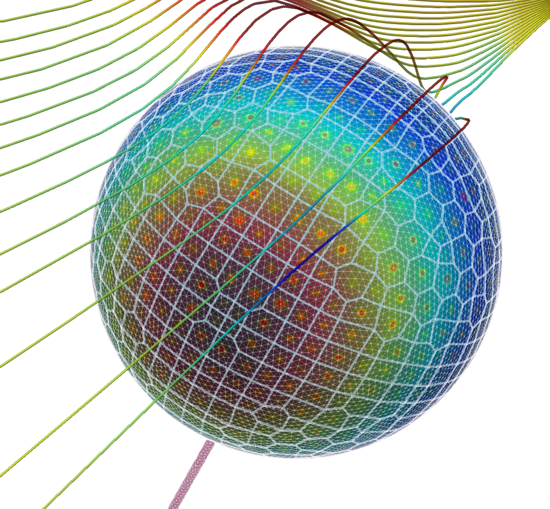
The computational mesh for CFD was created in an automated software module TMESH, using the snappyHexMesh open-source application. For each model component (in this case, just one component – Virtual Tunnel), a cartesian block mesh was created, as an initial background mesh, that is further refined along with the simulated object. The whole virtual tunnel is 20 m long, 7 m high, and 7 m wide. Basic mesh cell size is a cube of about 900mm edge. Three additional refinement regions are added. The mesh is gradually refined to the model wall. The mesh refinement levels can be easily changed, to obtain the coarser or finer mesh, to better handle the mesh size.Inflation layers can be easily handled. In this particular case, there are 8 inflation layers with an expansion ratio of 1.2. The final CFD mesh used for the simulation has in total 709,136 cells and consists mostly of hexahedrons.

The meshing application snappyHexMesh is not a compulsory meshing tool for TMESH at all. In case of need, any other external mesh can be loaded in TMESH directly in MSH, CGNS, or OpenFOAM format.

FEA mesh

The Computational mesh for CFD was created in an automated software module TMESH, using NetGen open-source application.

CFD Simulation Case Setup

The CFD simulation is managed with TCAE software module TCFD. Complete CFD simulation setup and run is done in the TCFD GUI in ParaView. TCFD uses OpenFOAM open-source application.

Simulation type: Virtual tunnel
Time management: steady-state
Physical model: Incompressible
Number of components: 1 [-]
Wall roughness: none
Inlet: Velocity 30 [m/s]
Outlet: Static pressure 0 [m2/s2]
Turbulence: RANS
Turbulence model: k-omega SST

Wall treatment: Wall functions
Turbulence intensity: 5%
Speedlines: 1 [-]
Simulation points: 1 [-]
Fluid: Air
Reference pressure: 1 [atm]
Dynamic viscosity: 1.8 × 10E-5 [Pa⋅s]
Air density: 1.2 [kg/m3]
CFD CPU Time: 2 core.hours

FEA Simulation Case Setup

The FEA simulation is managed with TCAE software module TFEA. Complete FEA simulation setup and run is done in the TFEA GUI in ParaView. TFEA uses Calculix open-source application.

TCAE Simulation run

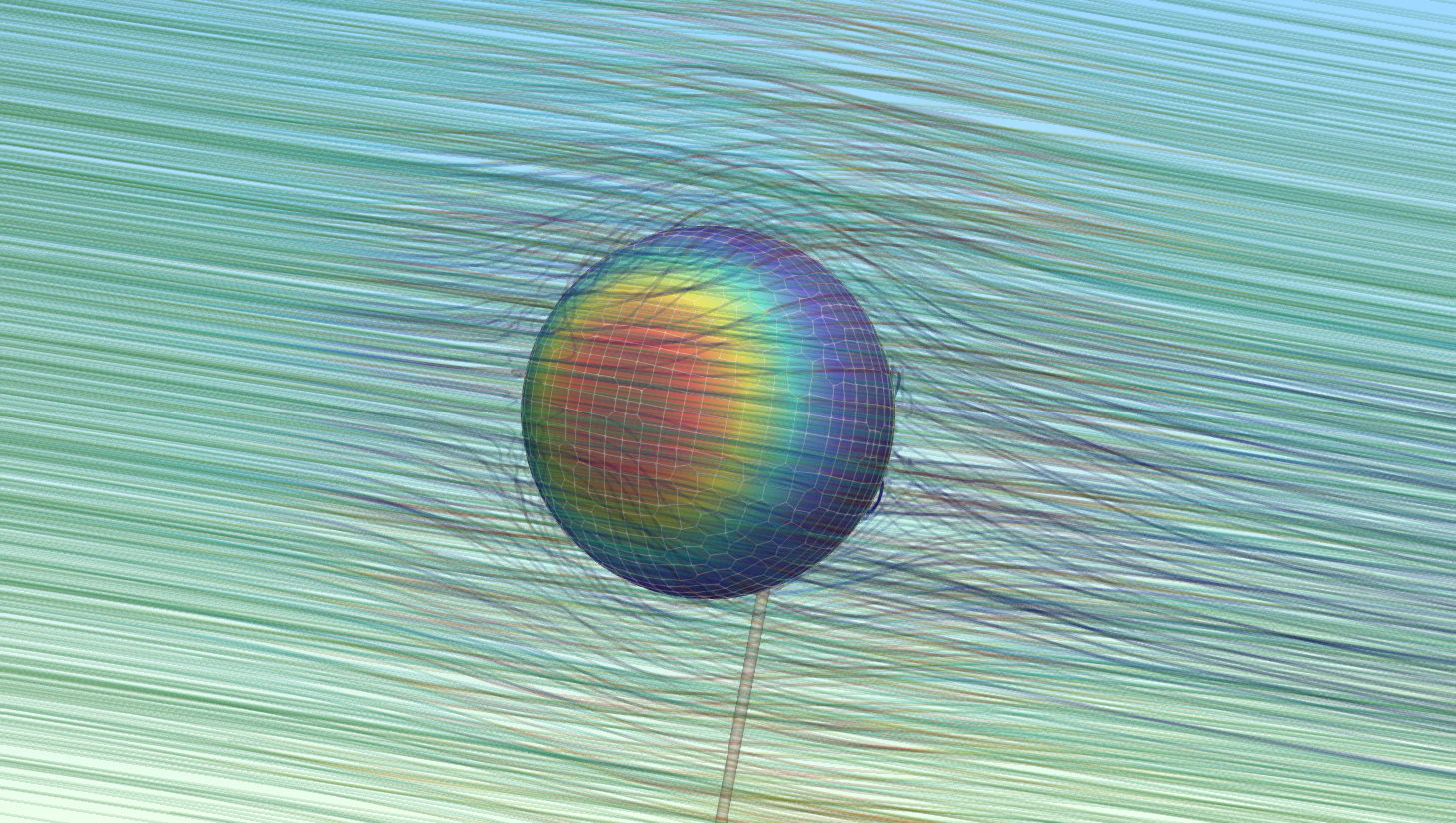
The simulation is executed within the automated TCAE workflow in steady-state mode, for one flow velocity value of 30 m/s. TCFD is capable of writing the results down at any time during the simulation. The convergence of any quantity is monitored during the simulation.

Results

Below is the final of the analytical solution with the simulation results.

Analytical solution Max Deformation [mm] = 26.60
TCAE simulation Max Deformation [mm] = 27.75

Analytical solution Max Stress [MPa] 83.78
TCAE simulation Max Stress [MPa] 92.48

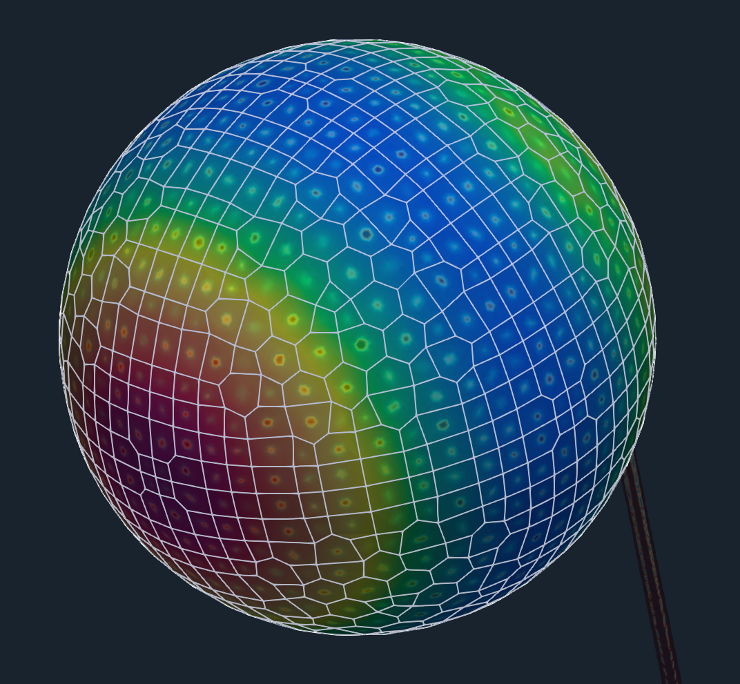
The compared results differ by less than 10% which meets well the original expectation. Despite the analytical 1d solution can be assumed as final, the simulation results can slightly differ according to the simulation settings. Especially, the CFD mesh and FEA mesh density may have certain effects on the simulation results. The following figures show the deformed beam stress magnitude and displacement magnitude. The deformation on the figures is ten times larger for a better visual perception.

Conclusion

The complex FSI analysis was performed successfully. It has been shown that the 3D TCAE simulation prediction gives a good agreement with the 1D analytical solution.
This benchmark is completely open, transparent, and repeatable. All the case data, resources and results are freely available. Everyone is welcome to contribute with new research about this case.
TCAE showed to be a very well suited tool for CFD, FEA, and FSI engineering simulations.
More information about TCAE can be found on CFD SUPPORT website: https://www.cfdsupport.com/tcae.html
Questions will be answered via email info@cfdsupport.com

References

[1] TCAE Manual
[2] TCAE Training
[3] Wikipedia https://en.wikipedia.org/wiki/Centrifugal_pump
[4] https://www.mechstudies.com/what-is-pump-basics-parts-types

[5] Drag of a Sphere https://www.grc.nasa.gov/www/k-12/airplane/dragsphere.html

[6] E.g. https://en.wikipedia.org/wiki/Moment-area_theorem

[7] On-line beam calculator: https://calcresource.com/statics-cantilever-beam.html

Flow Visualization

Download TCAE Tutorial - Beam-Ball FSI Benchmark

File name: beam-ball-FSI-benchmark-TCAE-Tutorial-21.09.zip

File size: 7 MB

Tutorial Features: CFD, FEA, FSI, VALIDATION, BENCHMARK, TCAE, TMESH, TCFD, TFEA, SIMULATION, BEAM, BALL, SPHERE, EXTERNAL FLOW, INCOMPRESSIBLE FLOW, DEFORMATION, DISPLACEMENT, STRESS, MODAL ANALYSIS, INCOMPRESSIBLE, RANS, AIRFLOW, STEADY-STATE, AUTOMATION, WORKFLOW

Beam Ball FSI Benchmark

Beam-Ball FSI Simulation Benchmark

PDF REPORT

CFD Simulation Report

FEA Simulation Report